In this article, we’ll examine ridge regression – a simple technique which is a great place to get started with machine learning and algorithmic trading. We’ll talk a bit about the technical details, and then backtest a ridge regression on some stocks with some excellent graphs to visualise where the algorithm decides to buy and sell, and where it gets it right and wrong.
With the spectacular progress made by AIs like ChatGPT recently, there might be renewed interest among casual and professional traders to explore using machine learning methods in their trading strategies. Some major trading firms publicly promote that they use machine learning methods, even though they don’t. However, machine learning can be more than good publicity. Done naïvely, machine learning can be prone to overfitting. That is, fitting to the idiosyncrasies of a piece of data in a way that will not hold outside of that dataset. However, done carefully, it can help you to evaluate whether there is any potential statistical significance in a signal, and help you find the optimal mathematical form of the buy/sell points for any signals you do have confidence in.
It’s important to realise that statistics as a field tends to assume that a mathematical (eg, scientific) relationship exists in the data, but is obscured by a certain amount of random noise. In trading, since decisions made by market participants are much less precise, and affected by unpredictable news events which are extraneous to any algorithm, it’s often not entirely possible to use backtesting to prove that a trading strategy will be profitable into the future. An exception could occur in high frequency trading where the use of algorithms by other participants could generate statistically detectable patterns. Caution, pragmatism and common sense are important here.

Among the simplest of machine learning methods is linear regression. It can be used as a starting point to test whether your chosen signals have predictive value, before exploring more sophisticated machine learning methods which may be more effective. There’s more than one way you might set up the inputs and outputs for a linear regression, but a straight-forward approach is to use the previous n (relative) price changes to predict the next price change (often called an autoregression). It’s interesting to note that a moving average crossover strategy considers whether a linear function of recent price moves (the short average minus the long average) is positive or negative. It is therefore a subset of the possible trading strategies that a linear regression can find.
You can then add to the past price moves your favourite signals such as moving averages or regression lines. You can even add in signals calculated from other assets that you believe may be related or correlated, in order to generate a kind of pairs trading or statistical arbitrage strategy (although this is a topic for another article!)
While our linear regression is attempting to predict the next price move, we need to convert this into a trading strategy. A simple buy/sell strategy is to buy when the predicted move is larger than some positive threshold, and sell when the predicted move is lower (more negative) than some negative threshold.
Ridge regression is a modification of linear regression which helps to prevent overfitting. It’s therefore particularly useful in the context of trading strategies.
Linear regression chooses a coefficient for each signal in a way that makes the predicted values as close as possible to the real values. Ridge regression modifies this by also trying to keep the coefficients small. The trade off between the two considerations is specified by a parameter ‘alpha’ that the user may choose. So, imagine that assigning one of our signals a large coefficient only improves the prediction very slightly. Linear regression will go ahead and assign the large coefficient, potentially giving a lot of weight to a signal that doesn’t have much predictive value, and what predictive value it has may be spurious. On the other hand, ridge regression will say, “this signal doesn’t improve the prediction very much, it’s better to make its coefficient close to zero.” The benefit to avoiding overfitting a trading strategy is clear.
With any autoregressive model, one should check that the data is “stationary” before fitting the model. This means that the statistical properties such as mean and variance do not change over time. In practice, differencing the data (i.e., working with the relative changes in the data instead of the absolute price values) is likely to result in sufficiently stationary data for our purposes.
It’s a good idea to standardize your signals to have mean 0 and standard deviation 1 before doing a regression. This means that the size of the coefficients are more comparable and help you quickly identify which signals are significant.
It’s common in machine learning to fit the model on one block of data (the fitting set), and evaluate it on another (the test set). This helps prevent overfitting to the randomness in a particular piece of data. However, keep in mind that your model could still overfit to idiosyncrasies that are common to both the fit and test sets, but which will not necessarily persist into the future (and it’s a good idea to use a stop loss when executing your strategy to deal with market behavior suddenly diverging from what was represented in the test and fit sets).
When using intraday data such as 1 minute or 1 hour data, it’s necessary to decide what to do about the gaps that occur at the start of a new trading day. A naïve approach is to simply join the data from each day together, but the sudden jumps in the data could negatively affect your regression. For one minute data, the jumps represent only a small portion of the data, and so one might get away with this approach for an initial analysis. The correct way to handle the jumps is to not try to predict the first n price moves of each new day, and remove these from your regression. Instead, the first prediction included in the regression should be the (n+1)th price move of the day.
A choice must be made on which frequency of the trading data to use. For example, one minute, one hour or one day. I tend to prefer short time intervals for two reasons. The first is that it results in a much larger number of data points. The second, is that behavior over shorter time intervals is more likely to be caused by algorithmic trading strategies, and therefore more likely to have statistically detectable patterns. However, momentum and mean reversion strategies driven by (human) market sentiment could also be effective over longer time periods.
Our strategy has a number of parameters. One is the alpha parameter in the ridge regression which controls the relativity between trying to get the closest fit for the predictions, and trying to keep the coefficients small. Another is the already mentioned threshold that determines when a predicted move is large enough to trigger a buy or sell action. Finding good parameters to use is a matter for experimentation. Alpha should be chosen so that it seems to use near-zero coefficients for any signals that are believed to be extraneous. Threshold determines the trading frequency, and if set too high could destroy profitability due to trading fees. If set too low, the strategy could miss out on profitable trades.
With the introduction out of the way, it’s time to look at the results!
I’ve written python code to grab data from Yahoo Finance, fit a ridge regression model to it, backtest the strategy and plot the results. I’ve chosen to use the ridge regression model that comes with the sklearn package, although there are others. I’ve used the lightweight_charts package to plot the trading data. It allows you to scroll and zoom through the candlestick data, and easily place buy and sell markers to visually represent the trading strategy.
For the purposes of this article, I’m going to keep it simple. My intent is to demonstrate the approach, rather than genuinely search for a successful strategy. The signals I’m going to include are the last 10 relative price changes, and moving averages and regression lines of lengths 5, 10 and 50 time steps. Exploring custom signals to include in the ridge regression could take us many places, and is best left for a future article. When backtesting, I’m assuming that after ‘selling’ the stock is being shorted, although it’s an easy change to assume we simply have no exposure during these period.
I’m going to use one week of 1 minute data, with approximately one day (the most recent day) being set aside as the test set.
In the graphs, the light blue line shows the ridge regression’s prediction of the next move. Remember though that we’re not exactly trying to predict the next move. Instead, the predicted move is used as an indicator of when to buy or sell. When the absolute magnitude of the predicted move is larger than some threshold, we buy or sell based on whether the move is up or down.
Normally, one might use something like p-values to gauge the statistical significance of each signal. When doing a ridge regression, which tries to make the coefficient small if a signal doesn’t significantly improve the prediction, we can use the size of the coefficients as a quick way to gauge which signals are important (although note this is not the same thing as statistical significance.).
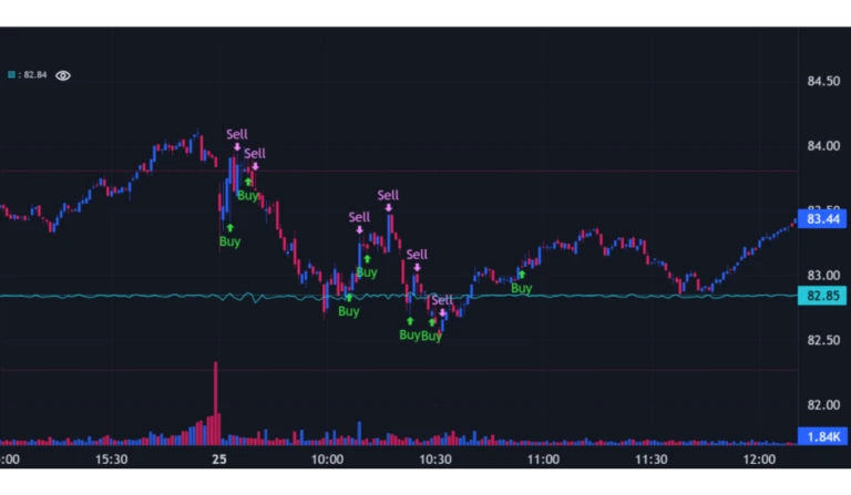
For no particular reason, let’s start by seeing how the ridge regression performs on Starbucks stock. The data comes from the week 21st-25th of April 2025. The below python output shows the coefficients (scaled by 1000) assigned to each of the signals and the strategy profit compared to buy and hold.
close_-10 = -0.07
close_-9 = -0.14
close_-8 = 0.00
close_-7 = 0.09
close_-6 = -0.01
close_-5 = 0.02
close_-4 = -0.03
close_-3 = 0.01
close_-2 = 0.03
close_-1 = 0.00
RegLine5 = -0.49
RegLine20 = 1.87
RegLine50 = 0.27
MovAvg5 = -0.47
MovAvg20 = -1.47
MovAvg50 = 0.23
Strategy profit = 2.77
Buy Hold profit = 0.97
In this case, the strategy is nearly three times as profitable as buy and hold. Of course, testing on other blocks of data would show different results, and some might show the strategy less profitable than buy and hold. Looking at the size of the coefficients, it appears that the 20 day moving average and 20 day regression line are most significant, with the regression lines and moving averages all being more significant than the last ten relative moves (close_-1 to close_-10).
Using the lightweight_charts package to plot the trading data and buy/sell decisions, most of the algorithm’s trades occur before 11am, with few trades for the rest of the day. If the algorithm is trading too often given the trading fees, it’s easy to increase the threshold parameter to reduce the trading frequency. It’s encouraging to see that the algorithm can at times be very good at placing buys at the troughs and sells at the peaks.
close_-10 = -0.04
close_-9 = 0.19
close_-8 = -0.11
close_-7 = 0.16
close_-6 = -0.07
close_-5 = -0.10
close_-4 = 0.44
close_-3 = 0.01
close_-2 = -0.07
close_-1 = -0.25
RegLine5 = -0.72
RegLine20 = -0.46
RegLine50 = 0.93
MovAvg5 = -0.62
MovAvg20 = 1.49
MovAvg50 = -0.66
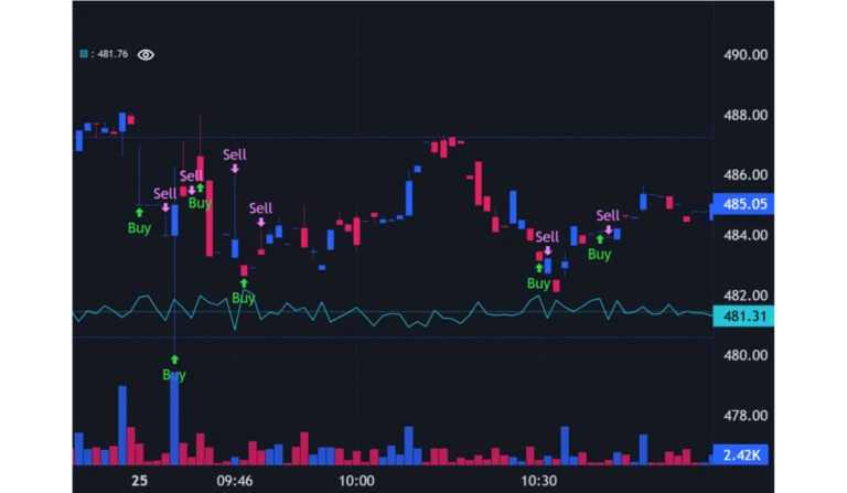
Strategy profit = 21.26
Buy Hold profit = 5.66
Again, the strategy is considerably more profitable than buy and hold (but I must reiterate that it should not be assumed that this will always be the case). Again we see the strategy is more profitable than buy and hold, with the regression lines and moving averages being most significant in the prediction. The algorithm trades mostly at the start of the day and the end of the day.
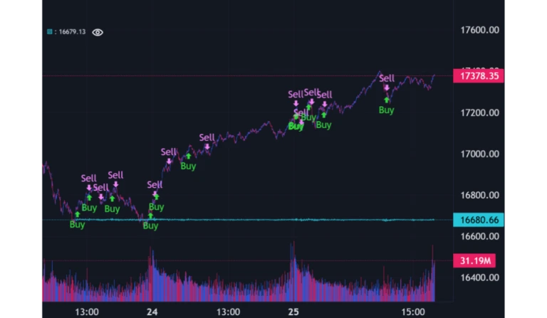
There’s a case to be made that algorithms on much more prominent assets such as major indexes are less likely to succeed than those on smaller or less traded assets, due to these assets being more “saturated” by traders (including big institutions) running algorithms. Let’s see how the algorithm performs on the most recent week of NASDAQ data.
close_-10 = -0.06
close_-9 = -0.09
close_-8 = -0.08
close_-7 = 0.19
close_-6 = -0.01
close_-5 = -0.09
close_-4 = 0.01
close_-3 = 0.03
close_-2 = 0.01
close_-1 = 0.02
RegLine5 = -0.10
RegLine20 = 1.06
RegLine50 = -0.38
MovAvg5 = -0.10
MovAvg20 = -0.38
MovAvg50 = -0.13
Strategy profit = -635.87
Buy Hold profit = 697.71
In this case, the strategy is less profitable than buy and hold, and actually loses money where buy and hold makes money.
Looking at the graph, the strategy is initially successful at selling at the top and buying again at the bottom. But as the NASDAQ begins a long climb, the algorithm interprets the noise around the trend as peaks and troughs and mistakenly buys and sells. I spent only a few minutes on this example, and it’s possible that more work and care could improve the outcome. But I intentionally made no attempt to adjust the parameters to achieve profitability here – I wanted to include an example where the strategy is not successful to add realism to the article and show the challenges that can occur. To be fair, it’s been a very volatile and unpredictable period for the US stock indices.
In this article, we’ve shown how a simple machine learning algorithm can be trained on stock data and used to generate a trading strategy. We’ve seen that even a basic approach can yield some encouraging results, but that there are also challenges. A trader wishing to pursue this approach further could now begin experimenting with different assets, a large number of different trading signals, and strategy parameters.
Genius Mathematics Consultants provides quantitative support traders and financial services firms including algorithmic trading, derivative pricing and risk modelling.
1. Lorem ipsum dolor sit amet, consectetur adipiscing elit. Ut elit tellus, luctus nec ullamcorper mattis, pulvinar dapibus leo.