There’s been some research into the prospect of using neural networks to price derivatives, such as options. Mathematical models to value derivatives are often slow, requiring computationally expensive numerical methods like finite differences or Monte Carlo. Since financial institutions can have an enormous number of live derivative trades, this makes revaluing the whole book challenging. Particularly if it needs to be done rapidly (as in high frequency trading), or a large number of times (as in a market risk calculation, for example). The idea here is to fit a neural network to the inputs and outputs of these derivative pricing models. Although fitting the neural network is computationally expensive, it only needs to be done once. Once the neural network has been trained, evaluating the neural network on a set of inputs to price a trade is extremely fast, and much faster than the numerical models it has fitted to.
The well-known French firm Murex is a leading provider of trading and risk management software. Customers of Murex regularly need to value large portfolios of derivatives trades, either for live pricing or to do market risk calculations. Murex have also been investigating the benefits of using neural networks for derivative valuation. On a related topic, a lot of work has also been done in the banking industry to use neural networks to speed up very computationally expensive XVA calculations.
In this article, we’ll develop python code to price options using neural networks. We’ll use the PyTorch package to fit the neural network, which we’ll train using an Nvidia 4090. You can also use your CPU if you don’t have a solid GPU. The option pricing model we’ll try to fit is simply Black-Scholes. Normally, there’d be no point in using a neural network to replace the Black-Scholes equations, which are both simple and fast. But once the methodology has been perfected, a more sophisticated non-vanilla product, or a local or stochastic volatility model can easily be substituted (one simply replaces the test set with options prices generated by whichever model one wishes to fit). Still, the Black-Scholes formula has five inputs, so we are still attempting the relatively challenging task of trying to fit a function of five variables.
I used ChatGPT to quickly produce some basic neural network training code. I use the paid subscription, which is supposed to use more sophisticated models than the free version. But I found that, by itself, ChatGPT struggled to solve the challenges required to develop a method that works to high accuracy for any conceivable option parameters. It is of course often the case with AI generated code that human direction is still needed for anything more conceptually difficult. So I needed to take over and use my own conceptual understanding to resolve the issues that arose. While AI generated code is not perfect yet, the code it generates represents an excellent “skeleton” that can subsequently be further developed by a human, accelerating development times.
The initial code generated by ChatGPT using 1000 training epochs to fit a neural network to 300,000 randomly generated call options (of course, the case of puts would offer no additional challenges). The output below shows the performance of the neural network on 10 randomly selected options.
Option 1: S=73.43, K=40.67, T=0.78, r=0.0106, sigma=0.0154: True BS: 33.09, NN: 33.14
Option 2: S=78.34, K=85.28, T=1.13, r=0.0790, sigma=0.0981: True BS: 3.44, NN: 3.47
Option 3: S=34.37, K=46.58, T=0.12, r=0.0085, sigma=0.1598: True BS: -0.00000036, NN: 0.000081
Option 4: S=39.67, K=29.81, T=1.39, r=0.0317, sigma=0.1719: True BS: 11.30, NN: 11.34
Option 5: S=51.71, K=22.05, T=0.16, r=0.0350, sigma=0.4353: True BS: 29.79, NN: 29.82
Option 6: S=89.14, K=97.69, T=0.94, r=0.0308, sigma=0.1489: True BS: 2.90, NN: 2.98
Option 7: S=77.43, K=75.10, T=0.24, r=0.0706, sigma=0.1959: True BS: 5.02, NN: 5.11
Option 8: S=56.26, K=2.60, T=1.47, r=0.0338, sigma=0.3914: True BS: 53.78, NN: 53.83
Option 9: S=48.82, K=27.15, T=1.29, r=0.0387, sigma=0.3691: True BS: 23.41, NN: 23.45
Option 10: S=45.65, K=4.12, T=0.43, r=0.0462, sigma=0.5064: True BS: 41.61, NN: 41.64
It appears to fit very closely! And my experimentation suggests that getting it to fit even more closely is just a matter of training it on more data, for longer, and if necessarily increasing the size of the neural network.
But there’s a problem: the neural network was trained on options having spot and strike between 0 and 100. Look what happens if we use the neural network on parameters outside this domain:
Option 11: S=230, K=225, T=1, r=0.02, sigma=0.1: True BS: 14.49, NN: 21.16
The neural network has fit to the parameter domain it was trained on, and won’t work correctly outside this domain. Taking an example from FX options, considering that AUDUSD is about 0.6, while XAUUSD is currently around 3200, we definitely don’t want a model restricted to a particular range. Clearly, a more careful approach is needed. Although I tried to coax ChatGPT to fix the issues itself (and it did have many suggested improvements), I wasn’t immediately successful. I found it easier to step in with an approach based on my own conceptual understanding.
Note that the other inputs won’t have this issue, as interest rates, time to expiries and volatilities can be assumed to fall within reasonable ranges. In practice, you might not have any options with expiries larger than 10 years, volatilities above 100%, or interest rates larger than 10%. There are two possible approaches here: 1) fit on a sufficiently large range of values, and don’t attempt to price any options with parameters falling outside of these ranges, or 2) train on the logarithm of these variables, and use training ranges that span a few orders of magnitudes.
Another issue that’s important understand here is the so-called curse of dimensionality. Because the Black-Scholes function has five inputs, we need to fill a five dimensional space with data points. Consider that if we wanted to create a grid with just 100 possible values for each input, the total number of data points required to completely fill the space would be 100^5 which is already 10 billion data points. And if you have six or seven inputs, forget it. For this reason, it’s a good idea to try to reduce the complexity of the function the neural network needs to fit by exploiting symmetries, or your own knowledge of the problem.
You might think that scaling or normalizing the data might resolve the problem. However, a standard scaling of all variables to have mean and standard deviation of 1 isn’t going to work. Instead, I’m going to take the approach of looking for symmetries in the Black-Scholes formulae.
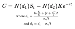
Looking at the form of the Black-Scholes equations, we see that the equation is invariant when spot and strike are divided by a common constant, while price is multiplied by that same constant. So let’s scale the input data so that spot is always 1. That is, we should divide spot, strike and price by spot. We’ll have to remember to multiply the output of the neural network by spot again to recover the Black-Scholes price. This transformation means that the neural network sees the “moneyness” of the option, rather than the specific spot and strike, and should help us resolve the problem of the limited domain we saw above.
Similarly, we notice that if we divide volatility by a constant, and multiply time to expiry by the same constant squared, then the price would remain the same apart from the discount factor. We could exploit this symmetry in our neural network fitting by separating out the discount factor as an additional input variable (so it is not modified when we scale time), setting the time to expiry to one, and dividing the volatility by the square root of t. Of course, having normalized all time to expiries to 1, there’s no point including them in the model. But actually, it’s a good idea to still leave the original time to expiry in there as an additional variable, because of the rt term in the expression for d1.
Of course, these manual considerations go somewhat against the spirit of having machine learning try to find the relationship by itself. Indeed, if you put the data through the Black-Scholes function before fitting, then the neural network only needs to fit the identity function. But these symmetries may continue to hold, or hold to a certain extent, when we begin using the code to fit more complex option pricing models. Let’s look at the results after these changes.
Option 11: S=230, K=225, T=1, r=0.02, sigma=0.1: True BS: 14.49, NN: 14.47
Option 12: S=125, K=130, T=1.5, r=0.02, sigma=0.11: True BS: 6.18, NN: 6.19
And you can see that the problem has been resolved, with our neural network now matching the Black-Scholes price for spots and strikes outside the original dataset!
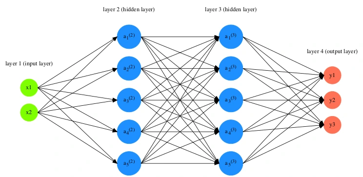
Here, I fit a network of 8 hidden layers, containing 256 neurons per layer, on 1.6 million data points (option prices). If we want the fitting to be even more accurate than this, it should just be a matter of training with more data, training for longer, or enlarging/changing the number of layers/neurons in the neural network.
Now that we’ve seen how Neural networks can replicate the behaviour of the Black-Scholes equations, a natural next step is to try to fit them to non-vanilla option models like barriers or American options. American options in particular are of interest, because the early exercise premium needs to be calculated using slow numerical methods. After that, we could start looking at more sophisticated volatility models, where the lightning fast speed of neural networks would be of great value. Keep an eye on the blog at www.mathematicsconsultants.com for some future articles on this topic, including the python code I’ve used.
Genius Mathematics Consultants provides quantitative support to traders and financial services firms including algorithmic trading, derivative pricing and risk modelling.
1. Lorem ipsum dolor sit amet, consectetur adipiscing elit. Ut elit tellus, luctus nec ullamcorper mattis, pulvinar dapibus leo.